- Syntax of the PV function
- Example # 1: Periodic Payments
- Example # 2: Single Payment
- Equalizing the rate and the period
- "By far this is the best training on the internet."
What is PV
We present value cashflows to see the value they’ll yield us in today’s terms.
It is mostly used as a decision-making technique by most investors, businesses, and companies. Let me tell you the practical applicability of the present valuing concept through a quick example.
Suppose you’ve signed a lease contract to lease a car. Per the contract, you’ve to pay $300 each year for 3 years as lease installments at a 10% interest rate 🚗
But what is the fair value of the car that you’re buying? If you’re doing the math like $300 * 3 = $900 – you’re doing it all wrong.
Since you are making these payments over 3 years and not today, they need to be discounted to today’s value. The fair value of the car you’re leasing is equal to the present value of the lease payments.
Discounting the lease payments in Excel, we get:
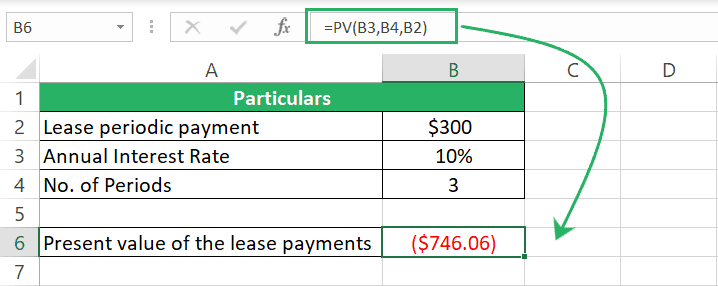
Hope this tells you the concept and importance of present valuing.
A stream of cashflows occurring at equal time intervals is called an annuity.

Kasper Langmann , co-founder of Spreadsheeto
How did we calculate the present value? Yes, that’s the next most important question. Get it explained in the coming sections 👇
How to calculate present value in Excel
Syntax of the PV function
The syntax of the PV function is as follows:
Click to copy Syntax Highlighter- Rate – the constant interest rate per period. The rate must be coherent with the payment period. For annual payments, supply the annual rate, for monthly payments, monthly interest rate, and so on.
- Nper – the total number of payment periods.
- Pmt (optional) – the periodic payment. If there are no periodic payments but any one payment only, omit the pmt argument and include the FV argument.
- Fv (optional) – this is the future value of the annuity at the end of the period. If omitted, Excel will assume fv as zero but, in that case, you must supply the pmt argument.
- Type (optional) – defined when the periodic payments are to be made:
0 or omitted – at the end of a period
1 – at the beginning of a period
Example # 1: Periodic Payments
Let’s take the same lease example as we discussed above to see how you can calculate the present value of equal periodic payments (annuity) in Excel.
Here’s a breakup of the major terms of your lease contract 📑
To calculate the present value of these lease payments in Excel
Step 1) Begin writing the PV function as below:
Click to copy Syntax Highlighter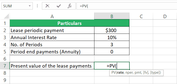
Step 2) For the rate argument, refer to the interest rate.
Click to copy Syntax Highlighter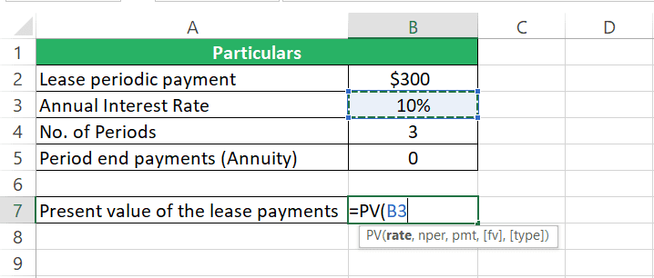
Step 3) For the nper argument, refer to the number of periods.
Click to copy Syntax Highlighter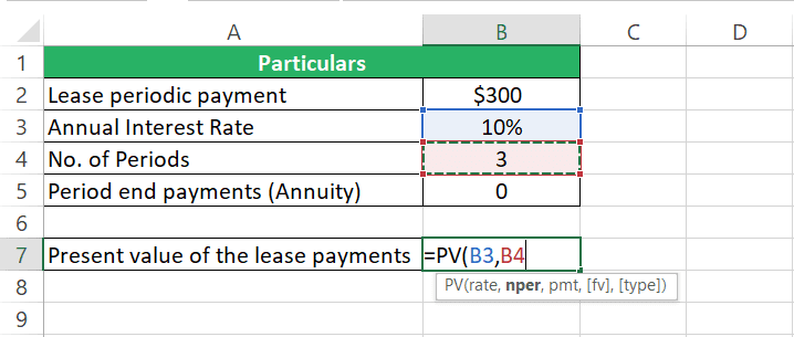
Step 4) For the pmt argument, refer to the lease payments to be made each year.
Click to copy Syntax Highlighter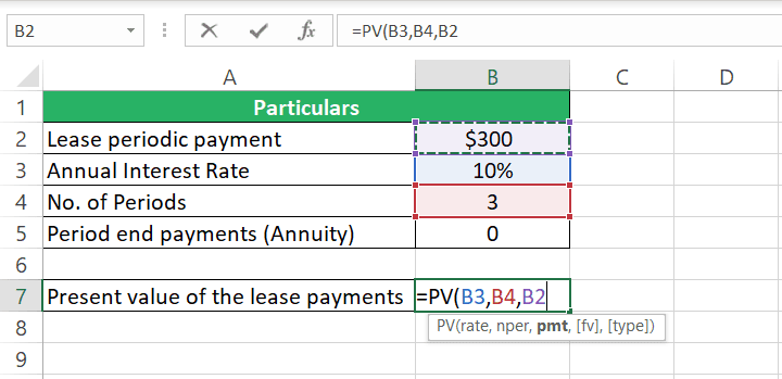
Step 5) We will omit the fv argument for this calculation.
Step 6) The lease payments are made at the [start-highlight]end of each period[end-highlight], so the annuity type is 0 (regular annuity). You can supply the type argument as 0 or leave it omitted)
Click to copy Syntax Highlighter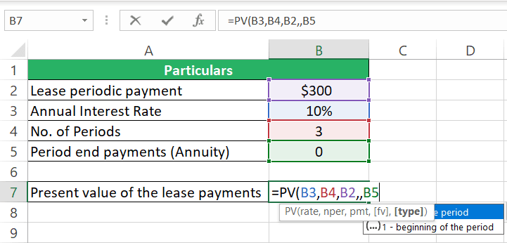
Step 7) Hit Enter to see the result.
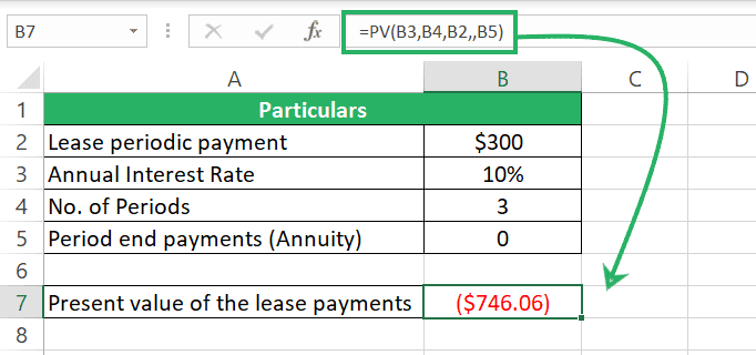
Excel returns the present value for this series of cash flows as $746.06.
This explains how easy and quick it is to calculate PV in Excel 😃
We calculated this present value as a regular annuity (with payments occurring at period end).
Had we done the same under the Annuity Due model (payments occurring at the beginning of the period) , the present value would have changed.
Click to copy Syntax Highlighter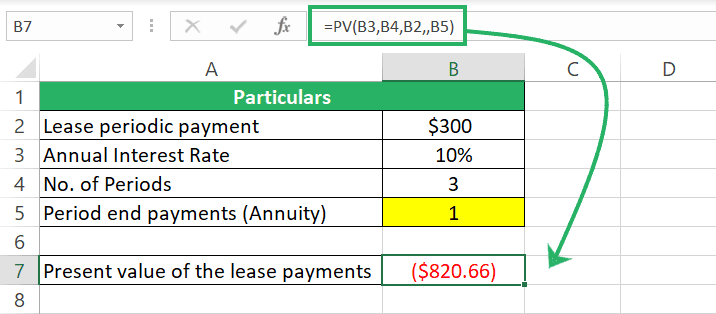
It is important to when each periodic payment is time to yield the correct present value of an annuity.
Pro Tip!
If a lease agreement starts from 01 January 2024 for 3 years until 31 December 2026:
Regular annuity means:
Payments occur at the end of each period i.e., on 31 December 2024, 31 December 2025, and 31 December 2026.
Payments occur at the beginning of each period i.e., on 01 January 2024, 01 January 2025, and 01 January 2026.
As the period when you’re paying cash varies, their discounting period varies, and ultimately the present value varies.
Example # 2: Single Payment
Except for periodic payments, you might also be in a situation where you want to calculate the present value of a single cash flow occurring at a certain point in the future.
Suppose you want to have $10,000 in your account after 3 years from now. If your account pays a 10% annual interest rate, how much money should you deposit in your account today to have 10,000 by year 3? 📆
The point to understand here is that $10,000 is a desired cash flow for Year 3. We will calculate its present value today by discounting it by 10% for 3 years.

Kasper Langmann , co-founder of Spreadsheeto
Step 1) Begin writing the PV function.
Click to copy Syntax HighlighterStep 2) Refer to the cell containing the interest rate / rate of return as the rate argument.
Click to copy Syntax Highlighter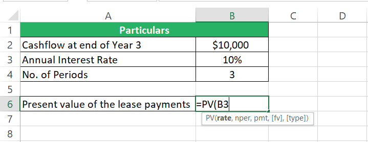 The fixed interest rate" width="719" height="278" />
Step 3) For the nper argument, refer to the number of periods after which the cash flow will occur.
Click to copy Syntax Highlighter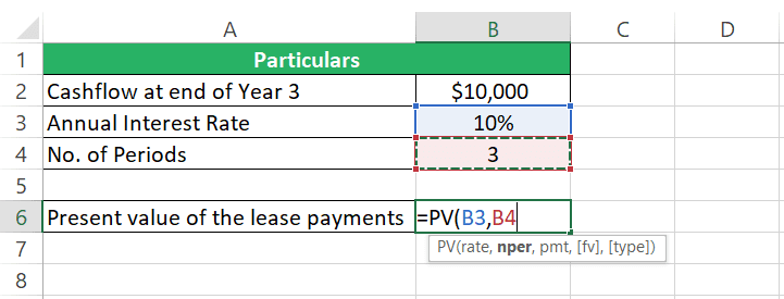
Step 4) Omit the pmt argument as there are no periodic payments.
Step 5) As the fv argument, refer to the future value we are expecting to occur at the end of Year 3 i.e., $10,000.
Click to copy Syntax Highlighter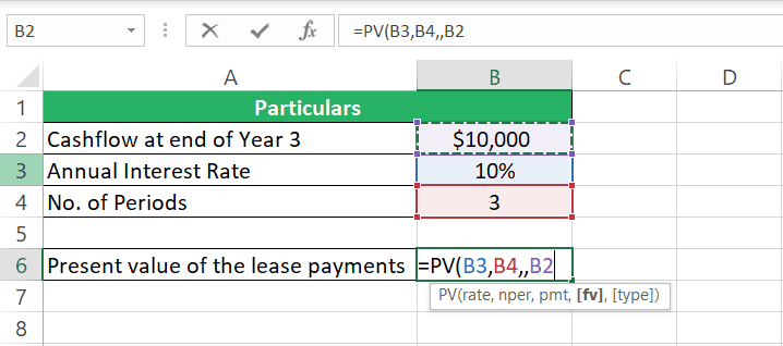
Step 6) Since there are no periodic payments, the “type” argument doesn’t matter here. The answer would be the same for type 0 and type 1.
Step 7) Hit Enter to see the result.
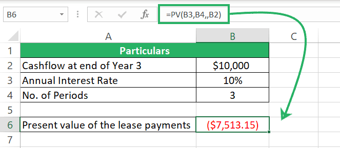
Excel returns the present value as $7513.15 💰
This is the amount that you must invest today in your account. It will sit there for three years and yield a 10% compound interest. By year 3, it would grow to $10,000.
Equalizing the rate and the period
Please note that while calculating present value, by period, we do not necessarily mean a year.
A period can be any length of time – a year, half a year, a quarter, a month, a week, or any number of days.
A period basically refers to when the periodic payments are being made and when the interest is being compounded on them ⌚
For example, if you’re paying $100 each month for 2 years and the interest rate is an annual 10%:
- The no. of periods is 24 (2 years into 12 months)
- There are 24 periodic payments of $100
- The applicable rate would be 0.83% (10% annual rate / 12 months)
The interest rate (rate) and the compounding periods (nper) must be coherent.
Here’s how you do it.
If you are making periodic payments of $100 for 2 years and the interest rate is an annual 10%, the change of compounding and periodic payment frequency must be catered to as follows.
To calculate the present value for periodic payments at monthly frequency:
Step 1) Divide the annual rate by the number of periods that fall in a year.
The annual interest rate of 10% means it would take your amount a year to yield a 10% interest. So how much interest would they yield in a week? 10% divided by 52 ➗
We do this to align the interest rate with the periodic payment/compounding frequency.
Click to copy Syntax Highlighter
Step 2) For the nper argument multiply the no. of years with the payment frequency each year.
We are making 52 monthly payments each year so, our number of periodic payments is 104.
Click to copy Syntax Highlighter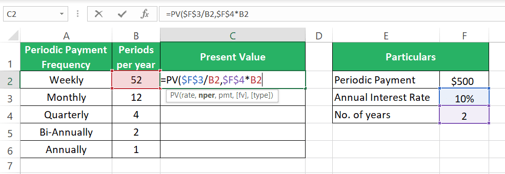
Step 3) Give in the pmt argument.
Click to copy Syntax Highlighter
And there are the results.
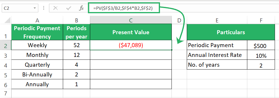
Step 4) I purposely used absolute references to be able to drag and drop the results.
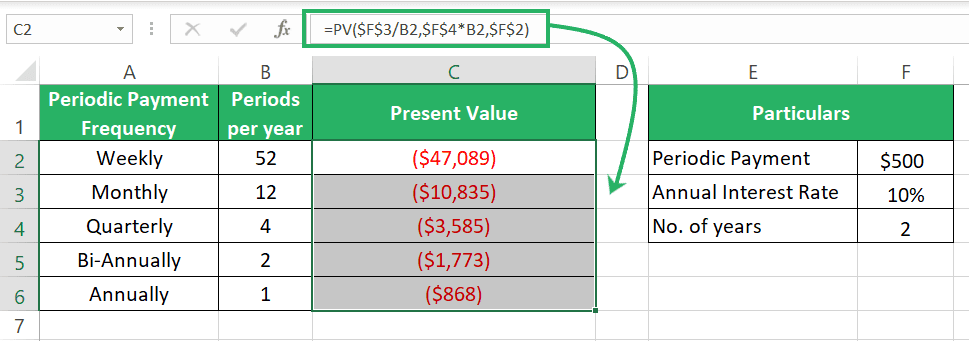
Always look out for the interval of interest rate – what is it? Annual, monthly, weekly, etc.
Then look for the periodic payments – how are they made? Annually, monthly, weekly, etc.
Accordingly, adjust the rate and nper to keep your calculations aligned 🚴♀️
Things to keep in mind
Playing around with the PV function is all safe when you know the following loopholes:
- The rate argument for the PV function must be supplied as a percentage (10%) or a decimal (0.1).
- Make sure the nper and the rate argument are coherent with each other. If you are making annual payments and the interest rate is also annual – all good. But if you are doing it any other way, ensure to adjust the rate and nper accordingly 🧐
- If you supply the pmt or the fv argument as a negative number, the output of the PV function will be a positive value.
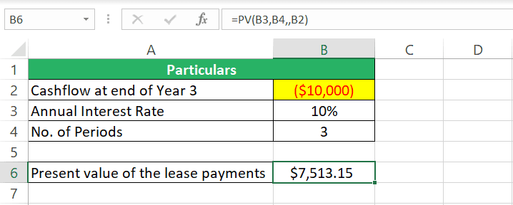
Inversely, if you supply the pmt or the fv argument as a positive number, the output of the PV function will be a negative value.
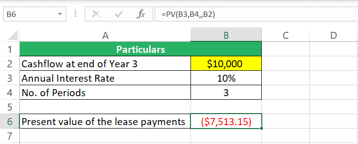
This is because Excel assumes a negative number as a cash outflow (something going from your pocket) and a positive number as a cash inflow (something coming into your pocket).
So, if you supply the fv argument as a positive number, this tells Excel that this value in the future is a cash inflow. To get a cash inflow of $10,000 in the future, you must invest cash of $7513 today (an outflow) 🎯
Therefore, it returns the present value of $7513 as a negative number if the FV is a positive number.
NPV vs. PV Function
The PV function of Excel can calculate the present value only for a similar set of cashflows.
As pmt you can only enter identical cash flows say $100 occurring at multiple intervals.
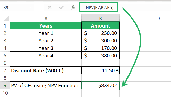
But if you have varying cashflows like $100 in Year 1, $200 in Year 2, $380 in Year 3, and so on, the PV function won’t be of help 🤔
For such a situation you’d need the NPV function.
The NPV function calculates the present value for varying cashflows that you can individually specify.
Conclusion
The PV function is one of the most used financial functions of Excel since present valuing is a very important corporate finance metric.
Present value is an essential finance concept as it helps determine the value of many assets and investments based on the returns and cash flows, they will potentially generate.
The PV function of Excel makes more sense when studied together with other top-notch financial functions of Excel including:
- How to Calculate Future Value in Excel (FV Function)
- How to Use Excel’s Annuity Formula (Example)